Add Line Of Best Fit Excel
Scatter Plots R Base Graphs Easy Guides Wiki Sthda

How To Add Best Fit Line Curve And Formula In Excel
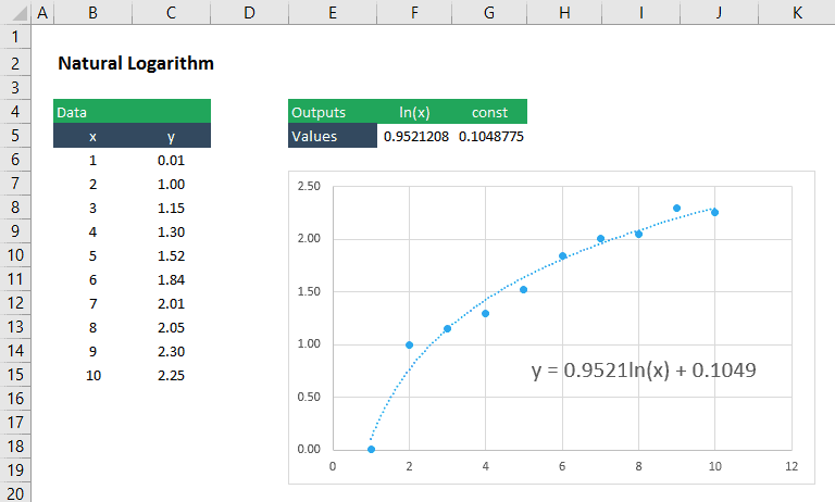
Nonlinear Curve Fitting In Excel Engineerexcel
Add A Linear Regression Trendline To An Excel Scatter Plot
How To Add Trendline In Excel Mac
Scatterplot With Fitted Regression Line Excel
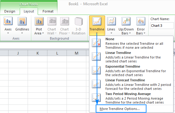
Trendline Options In Office Office Support
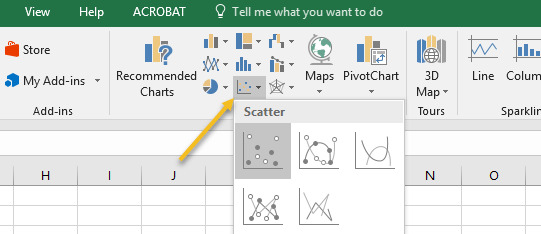
Figure 2 highlight the area with the data.
Add line of best fit excel. If you select a chart that has more than one data series without selecting a data series excel displays the add trendline dialog. Supposing you have recorded the experiments data as left screenshot shown and to add best fit line or curve and figure out its equation formula for a series of experiment data in excel 2013 you can do as follows. How to add line of best fit. We will select the range of cells that we want to chart and add a best fit line to.
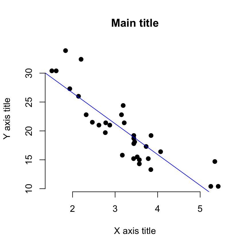
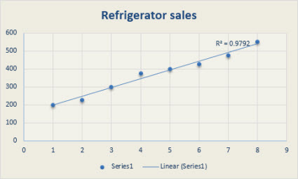
Learn how to plot a line of best fit in microsoft excel for a scatter plot. When drawing the line of best fit in excel you can display its equation in a chart. We will click on charts. Excel will then draw the chart in a new sheet in the current workbook and place me on that sheet.
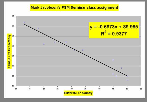
On your scatter plot select any data point and right click the data point to find an option that says add trend line. A logarithmic trendline by using the following equation to calculate the least squares fit through points. In our case please select the range a1b19. To start this process select the chart menu option and the add trendline menu suboption.
Where m is the slope and b is the intercept. The y values were specifically chosen to be inexact to illustrate what you will see when you analyze data from your labs. Y x a linear graph. How to create graphs with a best fit line in excel.
Open excel and input. Additionally you can display the r squared value. Now the task is to add the best fit line. Figure 1 how to insert best fit line.
To calculate the least squares fit for a line. And y x a non linear graph. It will look something like the screen shot below. In our case it is a2b21.
R squared value coefficient of determination indicates how well the trendline corresponds to the data. Excel calls this a trendline. Be sure you are on the worksheet which contains the chart you wish to work with. When working with more than one set of data points it is advisable to label rows and columns.
2in this manual we will use two examples. Where c and b are constants and ln is the. After creating a chart in microsoft excel a best fit line can be found as follows.
